What is A/B tests?
Imagine that you are running an e-commerce platform which is an otter plush specialty store. You find that around 20% of users cancel the transactions in the very last step of the checkout flow (Figure. 1-A). To improve the checkout completion rate, you come up with an idea that adding an adorable otter image (Figure. 1-B), which assumes that visual stimulates users to have stronger desire of purchase.

Figure 1. Otter Store Checkout Page
How do you know an otter image can actually boost the purchase? The naive way is just add it and observe the checkout completion rate. However, it is difficult to make the judgement regardless of the observation. For example, the increment might be affected by a popular video documenting how new born otters open their eyes (European Otter Brothers Open Their Eyes in Taipei Zoo). In other words, several factors influence the metric (i.e. checkout completion rate) you are observing.
It is necessary to make every conditions have equal average impact across variants (control and treatment) if you want to make the correct decision. In fact, the concept is the same as “controlled experiments” you may hear it several times in your life. In industries, A/B tests is a more prevalent term to describe the process of conducting a controlled experiment. A simplified process of A/B test consists of randomization, collecting data, and making statistical inference.
Take the same example, first of all, you randomly split half of users to experience the view with the otter image while the other half experience the current version. Secondly, collect the users data until it is enough to make a valid inference. Finally, compare the metric of interest. This process is demonstrated in Figure. 2.

Figure 2. Simplified A/B Test Flow
For further details, I highly recommend an article from Netflix TechBlog — “What is an A/B Test?”. It explains the idea of the A/B test and the importance of the A/B test. To conclude this section, I would like to quote an inspiring sentence in the article “Decision Making at Netflix” —
Making decisions is easy — what’s hard is making the right decision.
Frequentism and Bayesianism
The final step of an A/B test is to compare the metric (Figure. 2). Let’s say you observe the checkout completion rate of the view with an otter image is 84% and the one of the current version is 82%. It is indecisive only based on these two numbers because the results are always possible just driven by chance. The gap between the observed metrics and conclusion is so-called statistical inference (Figure. 3).

Figure 3. Statistical Inference
There are two common frameworks to perform the statistical inference — Frequenitsm and Bayesianism. In this section, I will introduce the notion of them without reaching unnecessary mathematics.
Frequentism
If you had taken any level of statistics courses, the course may remind you of numerous confusing statistical terminology like p-values and confidence interval, which are the concept based on the Frequentism. Frequentist approach is introduced by most of beginner level statistics course. Therefore, in fact you have already known it if you just suffered from your painful memory of statistics course.
In the world of Frequentism, it assumes that the reality is that there is no difference between the current (control) and revised version (treatment), which is called null hypothesis. In order to prove that the revised version is better, the strategy is to show that “it is highly unlikely to observe this A/B test results if the null hypothesis is true”. The p-value is one of the computation of this strategy, showing that the probability of observing your A/B test results (or more extreme) given that the control and the treatment is equivalent in terms of the metric of interest. It is conventional to set the threshold of rejecting the null hypothesis as 5% (significance level).
Set the significance level to 5% for the difference of conversion rate between the control and treatment (i.e. 2% in our example), it can also creates the other computation for this difference, 95% confidence interval, which says that if we repeat the A/B test, this interval will cover the true difference 95% of the time. If the 95% confidence interval doesn’t include 0, it shows that most of the time the treatment is better than the control. Hence, we can reject the null hypothesis that there is no difference between the control and the treatment.
Bayesianism
In the world of Bayesianism, it uses a distribution to describe the metric (or parameter). For example, we are 90% sure that the conversion rate is between 0.75 and 0.85 and 95% that it is between 0.7 and 0.9. Before starting an A/B test, an existing belief (prior) of the conversion rate should be contructed. During the process of collecting data, you continuously integrate new information and adjust your prior to form the posterior, the belief of the conversion rate after you see the data based on your prior.
To formulate the distribution of the conversion rate, Beta distribution describes this situation well. Figure. 4 demonstrates the reason why it is suitable in the case of the conversion rate. It is clear to adjust the parameters to form a belief in terms of the value and intensity. For instance, the red and blue distribution show that we believe that the conversion rate is around 0.8 while the blue one has less confidence. The green one forms a totally different belief from the red one. If we have no idea about the conversion rate before running an A/B test, we can also construct an uninformative belief as the gray distribution.

Figure 4. Prior Distribution
Once forming the posterior of the control and the treatment, it can be utilized to develop a simulation, which generates more data to calculate the probability that the treatment is better than the control. Using the same simulated data, it can also compute the expected loss if we choose the wrong variant. The whole process is shown in Figure. 5.

Figure 5. Bayesian Process
Analysis Tools
In this section, I will introduce one very powerful Python library to perform the analysis — Spotify Confidence. Spotify Confidence provides several powerful methods to easily and conveniently compute statistics like p-value and confidence interval, and moreover, create beautiful visualization of the A/B test results. Before we get started, I strongly recommend you to watch this video that explain the origin and the usage about Spotify Confidence library. In this section, I will use the same example throughout this article and show you how to use Spotify Confidence to analyze after data collection.
Frequentism
First of all, you have to import two required libraries, pandas and spotify_confidence. Also, to perform the analysis process, we create a clean and artificial dataframe as Figure 6.
import pandas as pd
import spotify_confidence as conf

df = pd.DataFrame(
    {
        'variant': ['control', 'treatment'],
        'conversion': [1230, 1302],
        'total': [1500, 1550]
    }
)

df.head()
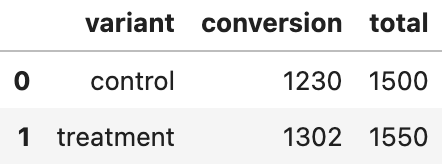
Figure 6. Exemplary A/B Test Results
One of the most common statistical significane tests is two-sample Student’s t-tests. There are 6 input variables required to initiate a StudentsTTest class. It is very straightforward to set all inputs. Notice that since the outcome variable conversion is binary, we set the input numerator_sum_squares_column the same as numerator_column. Also, notice that the type of categorical_group_columns is a list, implying that it is able to compare the subgroups results.
The experiment class in Spotify Confidence several common methods like summary(), which computes the point estimate and the confidence interval.
ttest = conf.StudentsTTest(
    data_frame = df,
    numerator_column = 'conversion',
    numerator_sum_squares_column = 'conversion',
    denominator_column = 'total',
    categorical_group_columns = ['variant'],
    interval_size = 0.95,
)

ttest.summary()
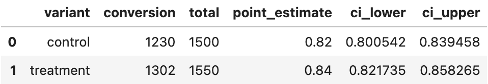
Figure 7. The t-test Results Summary
To see the difference between the control and the treatment, we simply use the difference() method and input groups to be compared. It returns a dataframe that contains calculated statistis like p-value and the upper/lower bound of the confidence interval.
ttest.difference(
    level_1 = 'control',
    level_2 = 'treatment'
)

Figure 8. Difference Summary
Besides statistics numbers, it is simple to visualize the results by the method difference_plot(). In our example, it shows that the confidence interval includes the value 0, representing that the results do not have enough evidence to reject the null hypothesis in 5% significance level.
ttest.difference_plot(
    level_1 = 'control',
    level_2 = 'treatment'
).show()
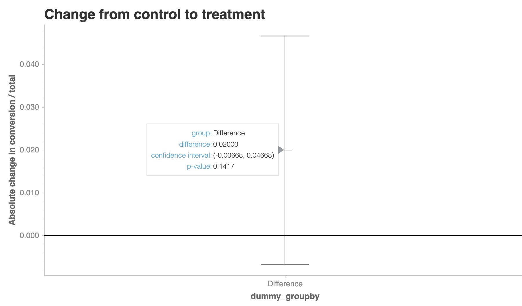
Figure 9. Difference Plot
Bayesianism
As introduced above, we can apply Beta distribution to form the belief in the case of conversion (Binomial). The inputs to initiate a class is almost same as Frequentist approach. You may notice that the values of ci_lower and ci_upper are different from what we found in the results summary of t-test. It is because Frequentist approach computes the confidence interval while Bayesian approach computes the credible interval.
bayesian = conf.BetaBinomial(
    data_frame = df,
    numerator_column = 'conversion',
    denominator_column = 'total',
    categorical_group_columns = 'variant'
)

bayesian.summary()

Figure 10. The beta-binomial Results Summary
My favorite part of Spotify Confidence is that it can create a concise and easy to understand chartify plot for Bayesian approach analysis. In this visualization, we realize the difference in terms of their distribution.
bayesian.summary_plot().show()
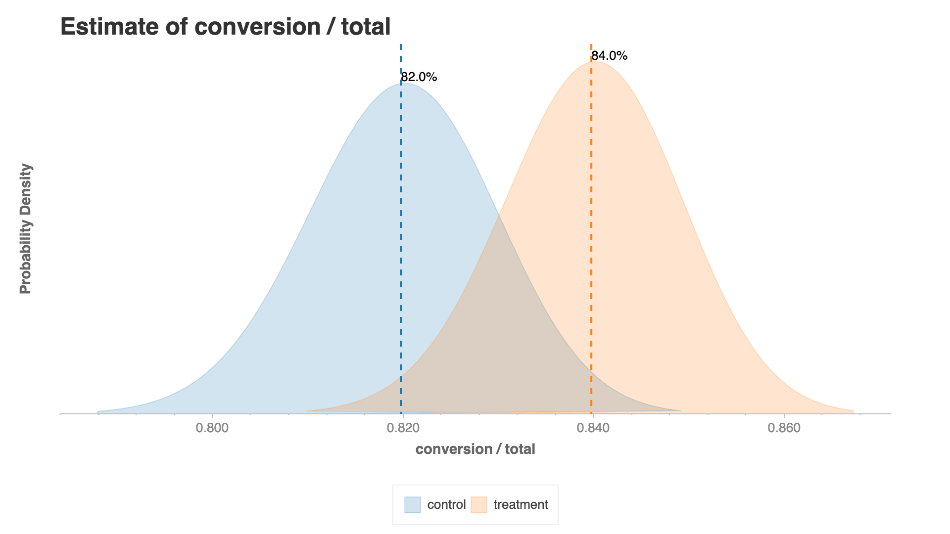
Figure 11. Bayesian Summary
The difference() method in BetaBinomial class simulates the results based on the distribution in Figure 11. and computes the difference, the probability that the treatment is better than the control, and the potential loss and gain across variants. Since the results are from simulation, we have to set the randomization seed for the reproductivity.
conf.options.set_option('randomization_seed', 1)

bayesian.difference(
    level_1 = 'control',
    level_2 = 'treatment'
)

Figure 12. Bayesian Difference
The difference_plot() method in Bayesian approach is very powerful. In this plot, we easily know the expected change from control to treatment and the probability that we make the wrong decision.
bayesian.difference_plot(
    'control',
    'treatment'
).show()

Figure 13. Bayesian Difference Plot
Summary
In this article, I introcude the concept and importance of A/B tests. To make a business decision from your A/B tests results, two statistical inference approaches are presented in the section Frequentism and Bayesianism. Finally, in order to execute the analysis, I demonstrate the basic usage of Spotify Confidence, a Python library for A/B test analysis.